Understanding The MCMC Algorithm - Part 1

July 15, 2020

In this next series of posts I will try to explain the ideas behind the Markov Chain Monte Carlo (MCMC) algorithms used in computer softwares and packages in order to compute the posterior distribution when using bayesian methods. I have learned about it by reading a great book by John K. Kruschke which can be found in this link.
This part will focus on the intuition and the main ideas underlying the Metropolis algorithm which is one algorithm of a larger family of MCMC algorithms. In future posts I intend to build on that intuition to explain additional material related to the use of MCMC in practice, let’s begin!

The Bayesian Framework And Why Do We Need MCMC?

In bayesian methods we assume something about the world and then use data to update our assumptions. So if there is a stream of data that we want to estimate its generating mechanism, i.e., the “function” that created this stream of data, we need to make an initial assumption about this “function” first, this is called our prior beliefs. Once we have our prior stated we proceed to observe the data and then update our priors accordingly. In the frequentist world view - this generating “function” has the same parameters each and every time it runs, in the bayesian world view the function’s parameters are random variables, i.e., they have a probability distribution. Bayes rule states that we can infer the distribution of the parameters $\theta$ of this “function” with the help of the data we observe $D$. $$P(\theta|D) = \frac{P(D|\theta)P(\theta)}{P(D)}$$

where $P(\theta|D)$ is called the posterior, i.e., our updated-by-data beliefs, $P(D|\theta)$ is called the likelihood and it represents the likelihood of the data given our beliefs. $P(\theta)$ is the prior. Finally, $P(D)$ represents the probability of the data over all possible beliefs, and it is usually thought of as a normalizing constant.

Calculating $P(D)$ requires us to compute the integral over all possible beliefs. In real applications this can be a very hard thing to do. In my previous post I wrote about conjugate priors and how easy it is then to calculate the posterior in a closed form using such priors. In real life applications it is rarely the case.

If we have only one parameter with a finite range to estimate, we can try to approximate the integral by grid approximation, but what if we have several parameters (which is the more common case)? In these situations we won’t be able to span the parameter space with a reasonable number of points. For illustration, let’s say we have six parameters that we want to estimate. The parameter space is then 6-dimensional that involves the joint distribution of all combinations of those six parameters’ values. Setting a grid that will cover $1000$ different values per parameter will involve $1000^6$ combinations of parameter values, a number that is too large for any computer to evaluate in a reasonable time. What can we do instead?

Motivating Example: The Island Hopping Politician

Suppose that there is an elected politician that lives on a long chain of islands. The politician wants to keep his influence and status on each island, so during his day he hops from one island to the next. The population on each island is different - there are islands with a lot of people on them and there are islands with less people on them. The politician is not stupid, he wants to visit the more populated islands more frequently so that he spends the most time on the most populated islands, and proportionally less time on the less populated islands.

But he has a problem: Despite he was elected, he doesn’t know how many people are there on each island, and he doesn’t even know how many islands there are. However, he has a group of advisors who have some minimal information gathering capabilities. When they are free of eating and drinking, they can ask the mayor of the island they are on how many people are on the island. And when the politician proposes to visit an adjacent island, they can ask the mayor of that island how many people are on that island.

The politician has a simple heuristic for deciding whether to go to the proposed island: First, he flips a (fair) coin to decide whether to visit the adjacent island to the right (east) or the adjacent island to the left (west), once he has a proposal he needs to decide whether to actually accept it. If the proposed island has a larger population than the island he is currently on, he definitely will go there. If, on the other hand, the proposed island has a smaller population than the one that he is currently on, he will go there in a “probabilistic” way. So for example, if the population on the proposed island is only half as big as the population on the island he is currently on, the probability he will go there is only 50%.

More formally, let us denote the population of the proposed island as $P_{\textrm{proposed}}$ and the population of the current island as $P_{\textrm{current}}$. The politician will move to the less populated island with probability $p_{\textrm{move}} = P_{\textrm{proposed}} / P_{\textrm{current}}$. The politician is not a robot of course so he needs a device that will help him to come up with this probabilistic move, this is why he does this move by spinning a fair spinner marked on its circumference with uniform values from zero to one. If the pointed-to value is between zero and $p_{\textrm{move}}$, then he moves.

A Random Walk

Suppose there are 7 islands which are indexed by the value of $\theta$, so the leftmost island is $\theta = 1$ and the rightmost island is $\theta = 7$. The relative population on each island is increasing with $\theta$ so $P(\theta) = \theta$. The uppercase $P()$ in this setting means relative population and not absolute and also not the probability mass. In simple words, the rightmost island has the largest population relative to the other islands, and the leftmost island has the lowest population relative to the other islands. You can think about other islands to the left of 1 and to the right of 7 as all having 0 populations. The politician can propose to jump to those islands, but the proposal will always be rejected because the population on those islands will always be lower (it’s 0!) than of the island he is currently on. We can rewrite the formula of $p_{\textrm{move}}$ to be $$ p_{\textrm{move}} = \min\left(\frac{P(\theta_{\textrm{proposed}})}{P(\theta_{\textrm{current}})},1\right)$$ So when $P_{\textrm{proposed}} > P_{\textrm{current}}$ then $p_{\textrm{move}} = 1$.

In order to illustrate the mechanism let’s say our politician starts on island number 4. He flips a coin in order to decide which direction to go - left, to island number 3, or right, to island number 5. The probability to go to island 5 is 0.5 because if it is chosen the politician will go there with probability of 1 because of the increasing nature of the populations’ relative quantity in our problem, i.e., $P(\theta = 5) > P(\theta = 4)$. So when a right move is proposed it is always accepted (except the edge case of populations zero as been discussed above). However, The probability to go to the left, to island 3, is equal to $0.5\times\frac{P(\theta = 3)}{P(\theta = 4)} = 0.5\times3/4 = 0.375$. If the proposal to go to the left is not accepted the politician just stays in the current island, in this case island number 4. This can happen with probability $0.5\times(1 - 3/4) = 0.125$.

The above process continues and the probabilities continue to be computed the same way at every time step. When we have a long enough record of where the politician has been, we can approximate the islands’ populations ($\theta = 1$ to $\theta = 7$) distribution by counting the relative number of times that the politician visited each island.

Proposed Algorithm

Here is a summary of our algorithm for moving from one island to the next. We are currently at position $\theta_{\textrm{current}}$, we then propose to move one position either to the right or to the left. We choose this by flipping a coin (with a 50-50 chance). The range of possible proposed moves, and the probability of proposing each, is called the proposal distribution. In our example this distribution is a simple one with only two values of 50% each.

After we proposed a move, we then decide whether to accept it or not. The acceptance decision is based on the value of the target distribution at the proposed position, relative to the value of the target distribution at our current position. In our example, the target distribution is the unknown distribution of the population across the islands. If the value of the target distribution is greater at the proposed position than in our current position - we move to the proposed position with probability of 1. We definitely want to go higher when we can. On the other hand, if the current position has greater value than the value at the proposed position, we move to the proposed position probabilistically - we move to the position with probability $p_{\textrm{move}} = P_{\textrm{proposed}} / P_{\textrm{current}}$ where $P(\theta)$ is the value of the target distribution at $\theta$. Notice that what matters for the choice whether to move or not is the ratio $P_{\textrm{proposed}} / P_{\textrm{current}}$ and not the absolute magnitude of $P(\theta)$. Thus, as we can see, $P(\theta)$ does not need to be normalized, which means it does not need to sum to 1 as a probability distribution must. In our example of the politician, the target distribution is the population of each island, not a normalized probability.

After proposing a move by sampling from the proposal distribution and after determining the probability with which we will accept the move, we then actually accept or reject a move by sampling a value from a uniform distribution over the interval [0,1]. If the sampled value is between 0 and $p_{\textrm{move}}$ then we make the move. Otherwise, we reject the move and stay in our current position. We repeat the process at the next time step.

How Is This Helping Us?

In the proposed algorithm we are required to be able to do several things:

Generate a random value from the proposal distribution to get $\theta_{\textrm{proposed}}$.
Evaluate the target distribution at any given position to compute the ratio $P_{\textrm{proposed}} / P_{\textrm{current}}$.
Generate a random value from the uniform distribution to accept or reject the proposal according to $p_{\textrm{move}}$.

By being able to do those 3 things we are able to do, indirectly, something that we could not do before (directly) which is to generate samples from the target distribution. Moreover, we can do this even when the target distribution is not normalized.

When we look at the target distribution $P(\theta)$ as the posterior proportional to $P(D|\theta)P(\theta)$ (look at the formula for bayes rule at the beginning), we can generate random representative values from the posterior distribution merely by evaluating $P(D|\theta)P(\theta)$ (the likelihood times the prior), without normalizing it by $P(D)$, which is what we wanted all along.

MCMC: Terminology

To make things clear, in this post we are talking about the Metropolis algorithm which is named after the first author of the paper that first presented it (Metropolis, Rosenbluth, Rosenbluth, Teller, Teller, 1953). This algorithm is part of a larger family of algorithms that are called Markov Chain Monte Carlo (MCMC).

When we generate representative random values from a target distribution we perform a case of Monte Carlo simulation. Any simulation that samples a lot of random values from a distribution is called a Monte Carlo simulation, named after the dice and spinners and shufflings of the famous Monte Carlo casino. The naming of such methods as Monte Carlo is attributed to the mathematicians Stanislaw Ulam and the great John von Neumann.

The Metropolis algorithm also generates random walks such that each step in the walk is completely independent of the steps before the current position. Any such process in which each step has no memory for states before the current one is called a (first order) Markov process, and a succession of such steps is called a Markov chain, named after the mathematician Andrey Markov.

Island Hopping Politician Code Example

Let’s simulate the politician example in Python. The full code is available in this Github repo which will contain all other code examples in this series of posts as well.

First, lets create the real island distribution.

import matplotlib.pyplot as plt

import random

from typing import List

MAX_ISLAND = 7
SEED = 101

# real theta (the islands)
real_theta: List[int] = [i for i in range(1, MAX_ISLAND + 1)]

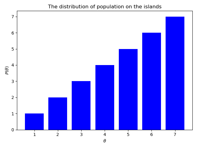
As was detailed in the example above, each island to the right has a greater value of the target distribution than the current island. The plot does not show the conceptual islands to the right of island 7 and to the left of island 1, but they are being accounted for in the code, as we shall see (their population is 0 so they will always be rejected).

Next, we define the function run_mcmc() that will run the random-walk simulation.

def run_mcmc(rounds: int, seed: int, islands: List[int]) -> List[int]:
    '''
    Runs the random-walk simulation `rounds` times
    and returns the resulting posterior distribution
    '''
    random.seed(seed)

    current: int = random.choice(islands)   # start somewhere
    proposal: int = 0
    n: int = len(islands)
    posterior: List[int] = [0 for _ in range(n)]
    round_count: int = 0

    while round_count < rounds:
        # determine which direction to take
        proposal_string: str = random.choice(['left','right'])
        if proposal_string == 'right':
            proposal = current + 1
        elif proposal_string == 'left':
            proposal = current - 1

        # condition for edge cases
        if (proposal > n) or (proposal < 0):
            proposal = 0

        p_move: float = min((proposal / current), 1)
        roulette: float = random.uniform(0, 1)
        if (roulette > 0) and (roulette <= p_move):
            current = proposal
        posterior[current - 1] += 1

        round_count += 1

    return posterior

Notice that if somehow the proposal is greater than the last island or smaller than the first island, then it is set to zero.
We count the number of times we visit each island by adding 1 at the relevant index position in the posterior list. This is true even if we stay at the same island (we just add 1 to the current island).

The following plots show the posterior for different number of rounds.

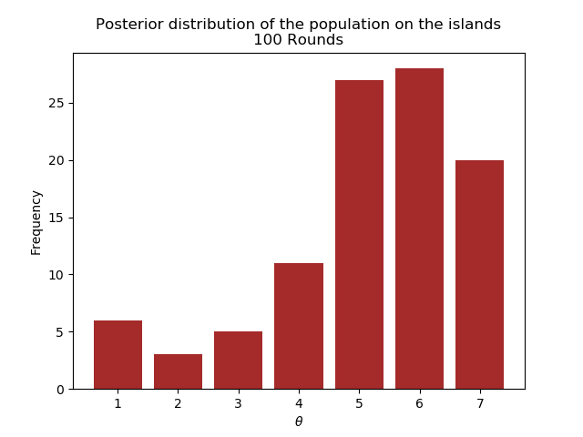
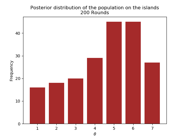
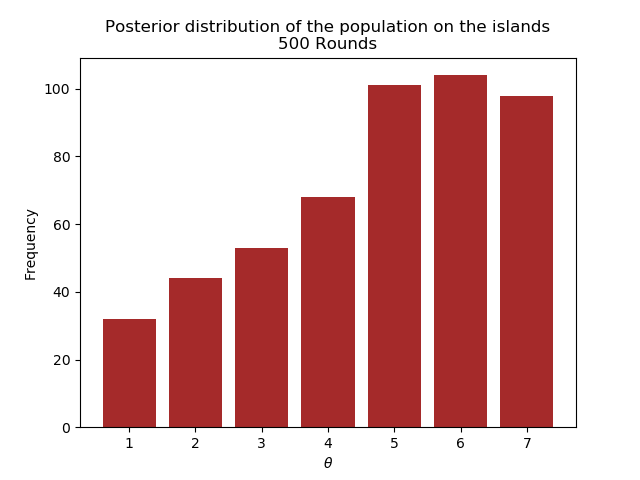
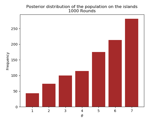
We see that after 1000 rounds, the posterior has converged closely enough to the real distribution.

MCMC More Generally

In the previous sections we described a special case of the MCMC algorithm that made it easy to understand how does it work. We considered the simple case of discrete positions (e.g. number of islands), one dimension, and moves that proposed just one position to the left or right.
The general algorithm applies to continuous values, multiple dimensions, and with more general proposal distributions.

The essentials of the algorithm are still the same. We have some posterior distribution, i.e. target distribution, $P(\theta)$, over a multidimensional continuous parameter space from which we would like to generate representative sample values. As before, we must be able to compute the value of $P(\theta)$ for any value of $\theta$. The distribution does not need to be normalized, it just needs to be nonnegative.

We generate sample values from the target distribution in the same way as before, i.e., by a random walk through the parameter space. We start at a random point which should be somewhere where $P(\theta)$ is nonzero. The random walk progresses at each step by proposing a move to a new position in the parameter space and then deciding whether to accept or reject the move. Proposal distributions can take many forms with the goal being to choose a distribution that explores the regions of the parameter space where $P(\theta)$ has most of its mass. In addition, we need to choose such a proposal distribution for which we have a quick way to generate random values.

After a new proposed position has been generated, the algorithm then decides whether or not to accept the proposal. The decision rule is the same - take the minimum of $P_{\textrm{proposed}} / P_{\textrm{current}}$ and 1 to get $p_{\textrm{move}}$. We then generate a random number from the uniform distribution on the interval [0,1]. If the random number is between 0 and $p_{\textrm{move}}$, the move is accepted. This process repeats itself, and in the long run, the positions visited by the random walk will closely approximate the target distribution (the posterior).

MCMC Applied to Bernoulli Likelihood and Beta Prior

Before wrapping up, I want us to take a look at another more “realistic” example of coin flipping. I have written about this example in the context of Multi Armed Bandit algorithms in this post.

In the previous island-hopping-politician example, the islands represented candidate parameter values, and the populations represented relative posterior probabilities. In this example of coin flipping where we are interested to find the underlying probability of the coin landing on heads, the parameter $\theta$ has values that range on a continuum from zero to one, and the relative posterior probability (the target distribution) is computed as likelihood times the prior.

When applying the Metropolis algorithm to this example we can think of the parameter values dimension as a dense chain of infinitesimal islands, and of the relative population of each infinitesimal island as its relative posterior probability density. Also, instead of being able to move just to the adjacent islands to the current position, the proposed move can be to islands farther away from the current island.

We will need a proposal distribution that will let us visit any parameter value on the continuum. We will use the normal distribution. The idea behind using the normal distribution is that the proposed move will typically be near the current position, and the probability of proposing a more distant position will drop off according to the normal (bell) curve. The magnitude of the standard deviation will highly affect the likelihood of a move to a distant position.

Flipping a Coin

We flip a coin $N$ times and observe $z$ heads, this is our data. We will use the Bernoulli likelihood: $$\begin{aligned} p(D|\theta) = p(z,N|\theta) = \theta^z(1-\theta)^{N-z} \end{aligned}$$ We start with a beta prior $p(\theta) = \textrm{beta}(\theta|a,b)$ (for reading more about using the beta distribution as the prior read my previous post). For the proposal distribution we will use the normal distribution with mean 0 and standard deviation (SD) denoted as $\sigma$. The proposed jump will be denoted as $\Delta\theta \sim N(0,\sigma)$ which means that it will be randomly sampled from the normal distribution. Thus, the proposed jump will be usually close to the current position, because the mean jump is zero. The proposed jump can be positive or negative, with larger magnitudes less likely than smaller magnitudes (governed by $\sigma$). The current parameter value is $\theta_c$ and the proposal parameter is $\theta_p = \theta_c + \Delta\theta$.

We then apply the Metropolis algorithm as follows: First, we start at an arbitrary initial value of $\theta$, in a valid range of course. This becomes the current value $\theta_c$. Then:

We randomly generate a proposal jump $\Delta\theta \sim N(0,\sigma)$ and denote the proposed value as $\theta_p = \theta_c + \Delta\theta$.
Compute $p_{\textrm{move}}$, the probability of moving to the proposed value $$\begin{aligned} &p_{\textrm{move}} = \min\left(1, \frac{P(\theta_p)}{P(\theta_c)} \right) \\ &= \min\left(1, \frac{p(D|\theta_p)p(\theta_p)}{p(D|\theta_c)p(\theta_c)} \right)\\ &= \min\left(1, \frac{\textrm{Bernoulli}(z, N|\theta_p)\textrm{beta}(\theta_p|a,b)}{\textrm{Bernoulli}(z, N|\theta_c)\textrm{beta}(\theta_c|a,b)} \right) \\ &= \ldots \end{aligned}$$ The last line is just replacing the relevant parts with the specific Bernoulli likelihood and beta distribution formulas.
Like we’ve seen in the Python example, if the proposed value $\theta_p$ happens to land outside of the permissible bounds of $\theta$, the prior and/or the likelihood is set to zero, hence $p_{\textrm{move}}$ will be zero.
Accept the proposed parameter value if a random value sampled from a [0,1] uniform distribution is less than $p_{\textrm{move}}$, otherwise reject the proposal parameter value and count the current value again.

We repeat the above steps until we see that a sufficiently representative sample has been generated. The issue of judging whether a sufficiently representative sample has been reached is not trivial and I hope to address this in part 2 of this series.

At the end of this process we should get the posterior distribution with it (hopefully) being a close representative of the underlying true distribution of the probability of heads.

Summary

In this post I tried to explain the main intuition behind the MCMC algorithms, specifically the Metropolis algorithm.
The problem with all bayesian inference methods lies in the difficulty to compute the integral of the normalizing factor in the bayes rule formula. The MCMC family of algorithms solve this difficulty by generating a representative sample of the posterior distribution.
In future posts of this series I intend to write more about further issues of the Metropolis algorithm and to present a new MCMC algorithm called Gibbs sampling. Thanks for reading!