Solving The Multi-Armed Bandit Problem with Thompson Sampling
Imagine that you are a data scientist working for a company that offers some sort of service by subscription. Let’s be more specific - your company offers an online LaTeX editor that everyone can use with some limitations: They cannot write long documents and they can’t use math notation, unless, they choose to sign up to your website and for a small fee of 10$ a month they get the access to all of your latex website features.
One day, The VP of design comes to you and says that his team have made some improvement to the toolbar of the editing window and they think that this will help the users to be more effective, thus increasing the sign-ups for you website. You are more skeptic, so you conduct an A/B test where you offer the regular-website version to a randomly selected group of your users, and the new-toolbar version to a second randomly selected group of users. You observe the sign-up rate for each group and conduct a statistical test which confirms that indeed, the new version “causes” more users to signup. You have increased your company’s revenues, and you and the VP of design give high-five to each other.
After a month, the VP of design knocks on your door once more. This time, he says that his team had produced several toolbar designs and they were not able to decide which version is better. He’s sure that you will be able to A/B test them all and find the best version that increases signups the most. Again, you are more skeptic.
Why A/B Testing With Multiple Variants is a Bad Idea
If you follow along the lines of a standard A/B test procedure when you have multiple variations that you want to test, you will probably start by comparing each variant against the control group, i.e., the group that gets to see the original non-altered website. There are couple of problems with that:
- With many comparisons, the probability of discovering at least one false-positive result, i.e., rejecting the null hypothesis when it is actually true, increases. The higher the number of variants to compare, the higher the chance of finding a false “winner”.
- It is not enough to compare each variant against the control to find the best variation. You will also need to compare each variant against each of the other variants. In this case, the number of tests increase and the chances of finding a false winner increase even more.
- Another reason why this is a bad thing to do is that you’ll need more data to conclude which is the winning variation, this in turn will lead you to run the tests longer. As the old saying goes: time is money. While you are conducting your tests you are loosing potential customers - these are the ones that get assigned to see the worse variants.
The Multi-Armed Bandit Problem
The problem our data scientist from the story above faces is a general problem of exploration vs exploitation, i.e., choosing the right ratio between exploring the different options and investigating each option in depth. These kind of problems are known as the Multi-Armed Bandit (MAB) problems. The origin of the name comes from the casino world, a place where a lot of statistical terms were firstly coined. The “bandit” is the slot machine which was called like that because it basically stole money from people. Each machine has an “arm” that the player pulls in order to start to play.
The MAB problem describes a person who comes into a casino and has limited time so he can play only $N$ games. He is facing a row of $M$ machines which all have different mechanisms so the probability of winning each one is different. The question is what should this person do? How many machines should he play and for how many rounds each in order to maximize his winnings?
A Bayesian Solution
Following up on point 3 above - what if there was a procedure which could choose the best variant at real time? Then we could offer the best variant to the users without loosing any potential signups. Well, it turns out that there is such a procedure and its called Thompson Sampling. But before I’ll describe this algorithm I want to review the core concepts of Bayesian analysis since Thompson Sampling utilizes these concepts.
Bayesian Analysis
In bayesian methods we assume something about the world and then use data to update our assumptions. So if there is a stream of data that we want to estimate its generating mechanism, i.e., the “function” that created this stream of data, we need to make an initial assumption about this “function” first, this is called our prior beliefs. Once we have our prior stated we proceed to observe the data and then update our priors accordingly. In the frequentist world view - this generating “function” has the same parameters each and every time it runs, in the bayesian world view the function’s parameters are random variables, i.e., they have a probability distribution. Bayes rule states that we can infer the distribution of the parameters $\theta$ of this “function” with the help of the data we observe $D$. $$P(\theta|D) = \frac{P(D|\theta)P(\theta)}{P(D)}$$
where $P(\theta|D)$ is called the posterior, i.e., our updated-by-data beliefs, $P(D|\theta)$ is called the likelihood and it represents the likelihood of the data given our beliefs. $P(\theta)$ is the prior. Finally, $P(D)$ represents the probability of the data over all possible beliefs, and it is usually thought of as a normalizing constant.
The great thing about bayesian methods is the fact that it really resembles human thinking. We all have our beliefs about something, and even when we don’t, we tend to make them on the spot (for instance if I were to hold my two hands as fists in front of you and say that inside one of them there is a coin, without knowing anything about me, you’ll probably say to yourself that there is a 50-50 chance for the coin to be inside each one of my fists). The weakest spot of bayesian methods is the choice of the prior. Some priors may allow us to compute the bayseian update in a closed-form formula, others will require the use of computational methods.
Thompson Sampling
The procedure of Thompson sampling is a simple iterative process:
- Assuming we have $M$ variants with unknown-to-us conversion rates $(\theta_1, \ldots, \theta_M)$, we randomly assign a value from the prior distribution for each one of these parameters. Think of these as the initial conversion rates.
- We pick the variant with the highest value.
- We offer this variant to the users and observe how many signed up and how many didn’t.
- We then take this new information and update our prior accordingly.
We repeat the above process until some stopping criterion is activated. For example it could be a fixed number of iterations that we had decided upon beforehand, or that a certain variant is “winning” for $x$ iterations in a row.
Choice of Prior
The main decision left for us to decide is the distribution we are going to use in order to mathematically represent our prior beliefs. Now since our outcome is a simple binary outcome (sign-up/not sign-up) a very common prior to choose which has several desired properties is the Beta distribution.
The Beta distribution is governed by two parameters $a$ and $b$, and depending on its values, the distribution can take on many shapes. The main reasons we want to use this distribution as our prior are:
- The Beta distribution is known to be a conjugate prior to the Bernoulli likelihood (the binary outcome we have). This means that when we calculate the posterior by multiplying the likelihood by the prior - we get a posterior which is Beta-distributed as well. This allows us to make the bayesian update more easily (mathematical demonstration coming up).
- The mean of the Beta distribution is equal to the proportion of positive cases (in a positive/negative binary outcome) which in our case is exactly what we’re after, i.e., the conversion rate (the proportion of sign-ups).
- Another feature of the Beta distribution is that if $a=1$ and $b=1$ the Beta distribution becomes the Uniform distribution which essentially assigns an equal probability to each item. This is desirable because we want to give each variant an equal chance of being the winning variant before we get any information from the users’ choices.
Mathematical Proof for Beta Distribution Being Conjugate Prior to Bernoulli Outcome
You can skip to the conclusion of this part if you are not interested in the mathematical details, it will not harm your understanding of the concepts being discussed here.
Lets say I want to check if a coin is fair. I observed $z$ heads in $N$ flips (this is the data).
My prior is Beta distributed:
$$\begin{aligned}
&P(\theta) = \frac{\theta^{(a-1)}(1-\theta)^{(b-1)}}{B(a,b)} \\
&B(a,b) = \int_0^1 \theta^{a-1}(1-\theta)^{b-1}d\theta
\end{aligned}$$
And my Bernoulli likelihood of the outcome I just observed is $\theta^z(1-\theta)^{(N-z)}$. $\theta$ is the proportion of heads.
Then by Bayes’ rule:
$$\begin{aligned}
&P(\theta|N, z) = \frac{P(N, z|\theta)P(\theta)}{P(N, z)} \\
&= \frac{\theta^z(1-\theta)^{(N-z)}\theta^{(a-1)}(1-\theta)^{(b-1)}}{B(a,b)P(N, z)} \\
&= \frac{\theta^{((a+z)-1)}(1-\theta)^{((b+N-z)-1)}}{B(a+z,b+N-z)} \\
&\sim \textrm{Beta}(a+z,b+N-z)
\end{aligned}$$
The conclusion is that we see that the update process is as simple as adding the number of heads we observed to $a$ and the number of tails we observed to $b$ - that’s it. This is what we will do in our procedure as well - e.g., if we observe 10 sign-ups we will add this number to our prior (Beta) distribution’s $a$ parameter and the same for non sign-ups for $b$.
Python Simulation
Let’s code these concepts to see if our intuition is correct. All the code can be found in my Github repo.
Note about reading the code: If you’ll try to read the code in the order it is presented here you’ll find that there are some parts that are actually being used before they have been defined so it is best to go back and forth across the different sections (or look at the github repo linked above). I am presenting it in this order for ease of explanation.
First we define an Environment class which facilitates running the simulation and saving states of important variables.
from __future__ import annotations

import numpy as np

from typing import Optional, Tuple, List


class Environment:
    def __init__(self, payouts: np.ndarray, variants: np.ndarray) -> None:
        self.payouts = payouts
        self.variants = variants
        self.variants_rewards: np.ndarray = np.zeros(self.variants.shape)
        self.total_reward: int = 0
        self.a_b_beta_prams: List[List[Tuple[float, float]]] =
        [[(1, 1) for _ in range(len(self.variants))]]

    def run(self, agent: ThompsonSampler,
            n_trials: int = 1000) -> Tuple[int, np.ndarray]:
        """
        Runs the simulation and return total reward from using
        the sampler chosen.
        """

        for i in range(n_trials):
            best_variant = agent.choose_variant()
            # mimick real behaviour
            agent.reward = np.random.binomial(n=1, p=self.payouts[best_variant])
            agent.update()

            self.a_b_beta_prams.append(
            [(a_i, b_i) for a_i, b_i in zip(agent.a, agent.b)])
            self.total_reward += agent.reward
            self.variants_rewards[best_variant] += agent.reward

        return self.total_reward, self.variants_rewards
This class can facilitate different samplers, not just the Thompson sampler, although it is the only one I have implemented here.
The payouts in the constructor is a Numpy array of the true conversion rates of the different variants (for the sake of simulation) and the variants variable is an array of variant indices.
Notice that in the run() method we model the decision of the customer of whether to sign-up or not by a Bernoulli trial with the probability of success being the underlying probability of the current best variant (updated from round to round). This does not mean that this variant will get more sign-ups necessarily. In expectation, it has a higher chance to get more sign-ups, but it might change as the simulation continues.
Notice also that like we said above, we are starting with a $(a,b) = (1,1)$ parameters for the Beta distribution to take a Uniform prior at the beginning, reflecting our lack of knowledge about which variant is better.
Next, we define a general Sampler class in order to be able to come back later and maybe add some more samplers’ implementations.
class Sampler:
    def __init__(self, env: Environment) -> None:
        self.env = env
        self.theta: Optional[np.ndarray] = None
        self.best_variant: Optional[int] = None
        self.reward: int = 0

    def choose_variant(self) -> Optional[int]:
        raise NotImplementedError

    def update(self) -> None:
        raise NotImplementedError
We want 3 things from a sampler - that it is connected to some environment, have a procedure to choose the best variant, and an update procedure.
The ThompsonSampler class is one such sampler.
class ThompsonSampler(Sampler):
    def __init__(self, env: Environment):
        super().__init__(env)
        self.a = np.ones(len(env.variants))  # prior of beta(1,1)
        self.b = np.ones(len(env.variants))  # prior of beta(1,1)

    def choose_variant(self) -> Optional[int]:
        self.theta = np.random.beta(self.a, self.b)
        self.best_variant = self.env.variants[np.argmax(self.theta)]

        return self.best_variant

    def update(self) -> None:
        self.a[self.best_variant] += self.reward
        self.b[self.best_variant] += (1 - self.reward)
It basically implements the update procedure we explained above (under the assumption that a Beta prior is being used).
With the definitions done, we turn to performing the simulation:
import numpy as np

from core import Environment, ThompsonSampler

from plot_funcs import plot_variants

# setup the "true" unknown parameters
pay = np.array([0.55, 0.04, 0.80, 0.09, 0.22, 0.012])
variants = np.arange(len(pay))

# perform the simulation
np.random.seed(1425)
env0 = Environment(payouts=pay, variants=variants)
samp = ThompsonSampler(env0)
env0.run(agent=samp, n_trials=1000)
(780, array([ 2., 0., 774., 0., 4., 0.]))
At the end of the simulation we get an output of the total reward, i.e., the total number of sign-ups, and the distribution of sign-ups across the different variants.
We can see that variant 2 (index 2 in the pay array, starting from 0) has the highest underlying conversion rate, but we also have variants 0 and 4 with somewhat high conversion rates as well. We can see from the output that almost all of the sign-ups in our simulation were done under variant 2 and very few under variants 0 and 4, so the results are consistent with the true rates.
Let’s plot the distributions after varying number of iterations:
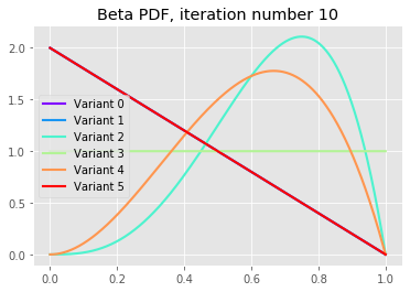
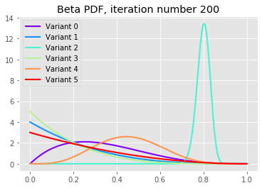
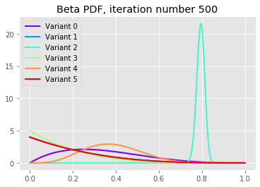
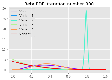
We can see that after 10 iterations variants 2 and 4 have large probabilities to sign-up, but as the iterations continue we see that the best variant, variant 2, is converging to its underlying probability with very small uncertainty (this is because we are in a simulation). Notice also that the poor variants have all fatter left tails indicating its low underlying conversion rates.
Conclusion
In this post we saw how can we utilize a Bayesian method, the Thompson Sampling procedure, in settings where we need to make a decision about which version of our product to go with among several different possible versions.
We saw that performing a regular A/B test has its drawbacks and in particular that it does not allow us to solve the exploration vs. exploitation problem in a very good way but using the Thompson Sampling procedure does.
Finally, we’ve constructed a simple simulation to illustrate these ideas.
Thanks for reading!